![]()
Pluto Occultation Observations on 14
August 2018
Dr. Donald Bruns, San
Diego, CA
dbruns@stellarproducts.com
Version created
August 25, 2018
Abstract
On the evening of August 14, 2018, Pluto slowly occulted a 13th magnitude star as seen from San Diego. Using a 28 cm aperture telescope with a CMOS camera, the photometric brightness of the combined star and Pluto was recorded over 27 minutes using 2 second exposures separated by 0.24 seconds. The brightness was calibrated by using six nearby reference stars in the same images, which compensated for some variable clouds that affected the raw measurements. The greatest dimming occurred at 10:32:19 pm PDT and the dimming lasted 116 seconds. This is 4 seconds later and 23 seconds longer than predicted.
1. Introduction
On August 14, 2018, a few hours after sunset in San Diego,
Pluto crossed in front of UCAC4-341-17633, a 13th magnitude
star. Since Pluto was about
magnitude 14.4, the total light from both targets dropped to about 20% of the
light before and after the occultation. A telescope was used to collect enough
light to record a time series of images. Pluto’s atmosphere scattered
some light as the star passed behind Pluto, so the dimming was not
instantaneous.
This photometric data was desired by the Lucky Star astronomical group headquartered in France, who coordinated the effort to get observers all across the shadow of Pluto as it crossed across North America (see figures in the Appendix). San Diego was about midway from the centerline to the edge, but Pluto was on the meridian at 35° altitude.
The equipment used for data acquisition is shown in Table 1. No color filters were included. The 1.7 arcsec seeing produced stellar images about 6 pixels FWHM. The sensor rows were oriented parallel to celestial Right Ascension. SharpCap was used to run the camera and MaxIm DL was used to process the images. Each image is time-stamped in the software at the time the exposure ended, so one second was subtracted to get the center time. There is an uncertainty of about 0.2 seconds because of the time stamping process, but this is negligible compared to the time seen in the occultation dip.
Table 1. Equipment parameters
|
Parameter |
Value |
Comment |
|
Telescope |
28 cm aperture |
Celestron Edge C11 at F/9.7 |
|
Mount |
German equatorial |
Software Bisque MyT
Paramount |
|
Camera |
CMOS monochrome, cooled |
ZWO ASI1600MM PRO |
|
Plate scale |
0.288 arcsec/pixel |
3.8 μm pixel, 2722 mm
focal length |
|
FOV |
23 x 17 arcmin |
4656 x 3520 pixels |
|
Image dead time |
0.236 seconds |
Download and save |
The night before the occultation, at about the same time, calibration images were recorded. Pluto was far enough from the target star that good relative brightness measurements could be calculated. This brightness ratio was used in the final data analysis.
To calibrate the camera and optical system, twilight flat field images were recorded on Aug 14. Since the camera was temperature controlled at -10 C, dark frames from August 13 were used. During the occultation, some low clouds started to appear which reduced the sky transparency. Fortunately, the sky was clear enough during the event to complete the data acquisition, and six reference stars surrounding Pluto were averaged to calibrate the data.
2. Dark field images
On August 13, 2018, 200 dark images were recorded by covering the telescope aperture during twilight (starting at 7:45 pm PDT, when the Sun was 3° below the horizon). Series were taken with the gain set to 200, 220, and 250, since the gain during the occultation was not yet determined. The exposure times were 0.012 sec (as used in the twilight flat frames) and 2 seconds (as used for the Pluto images). The 2 sec darks were taken starting at about 8 pm (Sun at -6°). The CMOS camera cooler was set at -10 C, using typically 25% power, so the temperature was stable. The actual temperature readout was noted as varying from -10 C to -10.5 C, an insignificant effect on the dark noise. The ZWO camera digitizes using 12-bits, and are automatically shifted two bits to get a range from 0 to 64k in 16 ADU steps. Each image file is 32MB.
All images were stacked using MaxIm DL software, with no alignment shift, using simple averaging. The saved files are considered master images, and were labelled DARK12msG200mean200, DARK12msG220mean200, DARK12msG250mean200, DARK2sG200mean200, DARK2sG220mean200, and DARK2sG250mean200. All master files are saved in FITS format, using IEEE Floating numbers, resulting in 64MB files. These are used to correct the image files taken on August 14, since the electronics are temperature controlled. Similar dark frames from August 12 had the same RMS noise.
Single image noises for the combinations are in Table 2. The noise does not diminish as the square root of the number of frames, so some fixed-pattern noise is present.
Table 2. Image noise for various exposure and
camera gain combinations.
|
Configuration
exposure (msec) |
Configuration
gain |
RMS noise
(ADU) in single image |
RMS noise
(ADU) in average of 200 images |
|
12 |
200 |
47 |
9.7 |
|
12 |
220 |
55 |
11.8 |
|
12 |
250 |
75 |
16.6 |
|
2000 |
200 |
55 |
20 |
|
2000 |
220 |
65 |
25 |
|
2000 |
250 |
89 |
35 |
3. Flat-field images
On August 14, 2018, flat-field images were recorded by pointing the telescope near the meridian at about 40° elevation just at sunset (first ones starting at 7:33 pm PDT). Starting with the 200 gain setting, a total of 200 images were taken. The gain was increased to 250 as the sky darkened. During the exposures, the telescope was moving at about 45 arcsec/sec in Declination (using the manual joystick). By the time each sequence was completed, the pointing was direction was shifted by more than a field of view, preventing any possible star buildup. The camera cooler was set at -10 C, typically using 25% power, assuring a stable temperature.
All images were stacked in MaxIm DL with no alignment shift,
using simple averaging. A master dark frame was subtracted to complete the
calibration. The files were saved as FLATG200E12ms_mean200,
FLATG220E12ms_mean200, and FLATG250E12ms_mean200. Figure 1 shows the resulting
flat field image (stretched for more contrast) and a horizontal profile through
the center. There is one dust donut
slightly left of center and a few smaller ones on the right side, but all are
far from any reference stars.
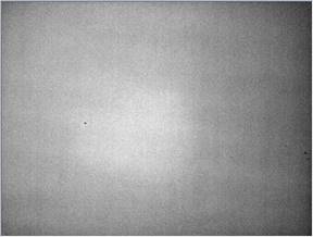
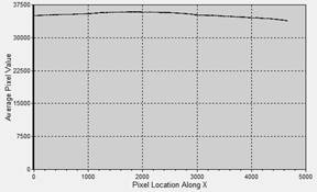
Figure 1. (Left) Flat field image, stretched to
show the uniformity across the field.
No dust shadows fell near the reference stars. (Right) A horizontal
profile plot near the center shows the signal at the edges falls only a few
percent compared to the center.
4. Pluto image
collection
After the flat field images were completed at 7:40 pm, the
telescope was idle until 8:45 pm. The telescope was centered on Pluto and the
pointing was not changed over the evening.
The telescope was carefully focused using magnitude 8.9 star
UCAC4-340-187047 using exposures about 0.2 seconds. This allowed a real-time display to ease
focusing through the turbulence. The air temperature was 69° F and stayed
at this number all during this first series. The reference star
UCAC4-341-187663 at magnitude 10.2 was then monitored for saturation, after
setting the exposure time to 2 seconds.
The gain was set so that this star was just under saturation, by
watching the display for about 100 frames.
It turns out that since the seeing was variable, some of the frames did
end up close enough to saturation that some non-linearity showed up, so this
star was not used in the final analysis.
The brightest reference star used in the final analysis was
UCAC4-340-187118 at magnitude 11.3.
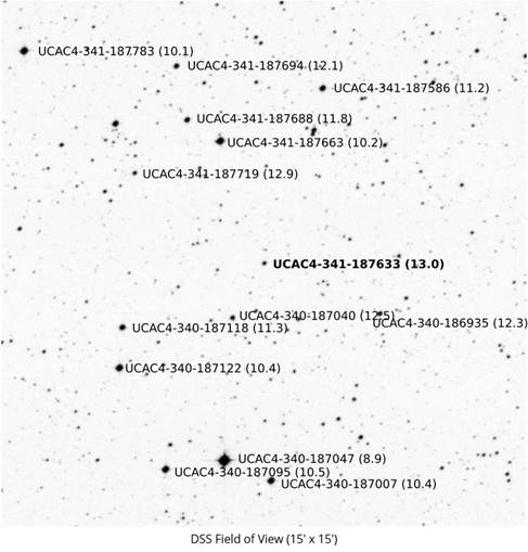
The first Pluto image series was started at 9:01 pm, when Pluto was about 15.5 pixels from UCAC4-341-187633, the occulted star. The intent was to use this series to measure the relative signals of the two objects to high precision, but as explained later, this series was only good enough to estimate the ratio. The seeing blurred the star and Pluto too broadly to allow better results. Nevertheless, 155 images (with 2 second exposures) were recorded using a gain of 200 and another series of 100 at a gain of 220. This imaging series ended at 9:10 pm.
Starting at 9:22, the same focus and gain tests were
repeated, with the image series starting at 9:31 pm and ending at 9:33 pm. The gain was set at 220, and the
temperature was stable at 69° F.
At 10:08 pm, the laptop was time-synchronized using Dimension 4 software that connects with an accurate internet time server. Some low clouds were approaching Pluto, so the camera gain was increased to 250. During focus and gain testing, the temperature was 68° F, and stayed at this value until the data collection ended. The image series started at 10:19 pm and ended at 10:46 pm. The occultation occurred at 10:32 pm, but the 27 minute long series allowed a better monitor of the cloud cover. It was too cloudy to take a planned series of images with Pluto on the opposite side of the target star one hour later.
5. Image corrections
The following steps were performed on every final Pluto sky image. The appropriate master dark image was subtracted while adding 1000 ADU to prevent negative values. The files were renamed by appending –dark. (For the flat fields, the additional 1000 ADU offset was not used.)
The flat fields were renormalized by dividing by the mean
(which was calculated over the entire image), resulting in nearly every pixel
varying between typically 1.04 in the center to 0.94 in the corners. In the central region, near Pluto and
the reference stars, the mean values vary between 1.00 and 1.02. These files were renamed to
FLATG200E12ms_mean200-meandark-normto1, FLATG220E12ms_mean200-meandark-normto1,
and FLATG250E12ms_mean200-meandark-normto1.
Every Pluto image was then divided by the appropriate normalized file. Because those dark-subtracted files had an additional 1000 ADU added, one more step was required. A constant image, where every pixel was set to 1000 ADU, was created and divided by the normalized flat field image. At the same time, an additional 1000 ADU was added to prevent negative values. Mathematically, this is explained by:
(RAW-DARK-1000)
- 1000
= (RAW-DARK)
NORM(FLAT) NORM(FLAT) NORM(FLAT).
Since the intensity of the target and reference stars are
determined in MaxIm DL by the sum of the pixel values inside a circular area
minus the mean value of the pixels in a surrounding annulus, the absolute level
is not important.
The flatness across a typical image is shown in Figure 2. The upper trace labelled “Raw” is a horizontal profile across the image, averaged over 20 pixels to reduce noise. One star shows up in the data. The curve is normalized to 1 and shifted up by 0.05 to show the general slope. The lower trace labelled “Raw/FF” is the same data with each pixel divided by the flat field curve, offset by -0.05. The shape is over-corrected because of the additional 1000 ADU offset meant to eliminate negative values. The middle trace labelled “Raw/FF-1000/FF” is the final result to which the photometry will be applied. This curve is very flat, as expected.
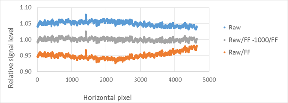
Figure 2. The flat field correction is shown by
horizontal plots of the normalized intensity for the raw image, an intermediate
image, and the final corrected image.
The final image is flat to better than 1%.
6. Integrated Signal
Measurements
MaxIm DL integrates the ADU signal inside a circle of radius R1, then subtracts the mean signal background determined from an annulus with outer radius radii R2. If the radii are too large, excess noise is added, so the optimum diameter was determined using several images with FWHM varying from 4.9 to 6.3 pixels. Tests were done on the target star (with Pluto just a few minutes before occultation) and a bright reference star. Varying the inner radius R1 while keeping the outer radius R2 fixed at 19 pixels resulted in the plot in Figure 3. With an R1 of 9 pixels, 95% of the integrated signal is captured, and that fraction varies only by about 1% over the different test stars. This is the radius used for all intensity analysis.
Figure 3. Increasing the aperture around a star
collects more light with the penalty of increasing noise. Using an aperture of
9 pixels collects 95% +/- 1% of the total light, and is the radius used in all
of the processing.
The process to easily copy the integrated intensities for hundreds of images in a series was the following. Every full image was opened and cropped and saved to a smaller image with 250x150 pixels dimensions, with the image center around one of six reference stars or Pluto. In this way, all 722 images in the time series could be opened at once, without computer memory problems. The MaxIm DL ALIGNMENT process was started, choosing “Auto one star”. The program took just a few seconds to align all of the images with respect to the first chosen reference image, using the bicubic interpolation option to estimate the new shifted pixel values. The process was closed, then re-opened, choosing “NONE” for alignment. The cursor was set at R1=9 and R2=19, simply advancing to the next image after manually copying the intensity value into an Excel spreadsheet. No realignment between images was needed, and the values are within 0.1% when compared to the original images.
7. Sky transmission
results
The relative sky transmission over the entire 27 minute occultation observation series was estimated by measuring the signal intensity of one nearby star (UCAC4-340-187118) in each of 722 images. At magnitude 11.3, its peak pixel was typically between 20,000 and 30,000 ADU, well within the linear range. The signal from the unresolved target star UCAC4-341-187633 and Pluto was also measured for each image. Both signals were normalized to 100% for the images taken about 700 seconds after the occultation, where the maximum transparency was seen. The results are plotted in Figure 4. The relative transparency dropped to about 40% at the beginning of the occultation, and rapidly increased to 75% during the occultation. Because several reference stars on both sides of the target star were measured, this drop should not affect the final results. The transmission was compared to images taken on the previous day, when no clouds were noted; the transmission was essentially identical. This means that the 100% level indicated in the figure represents a clear sky with some low-level haze.
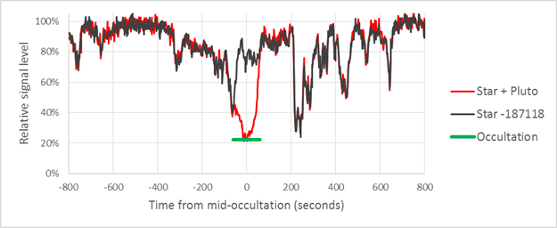
Figure 4. The change
in the sky transparency is plotted over a 1600 second period centered on the
occultation. The black curve is the
signal from a nearby reference star and the red line is the signal from Pluto
and the star it occulted. The time
of the occultation is indicated by the green bar. The signals are normalized to 100% at
700 seconds, where the transmission was greatest.
Images taken just before and after the occultation were analyzed to give a better mean value for the relative atmospheric transmission across the image during this critical time period. Since the clouds were moving, it was assumed that averaging the transmissions over several reference stars surrounding Pluto would reduce the noise and give a smoother result. These results are plotted in Figure 5, showing the relative transmissions for the six stars used in the analysis. The simple mean was used in the final analysis with no weighting by SNR, since the SNRs for each star were always much greater than 50.
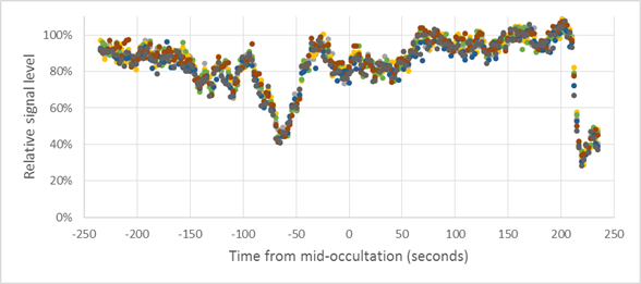
Figure 5. The relative
signal strength of six stars near Pluto was measured over an 8 minute period
centered on the occultation.
Averaging these measurements gives a better mean transmission factor.
With this mean transmission function, the signal levels for the six reference stars and the target star could be calculated. The results are shown in Figure 6. The intensity as a function of time is flat for all reference stars, as expected. The RMS of each star divided by the mean level ranges between 0.023 and 0.030, with an average RMS/mean of 0.026. This is for data at the 2.24 second recording rate, not smoothed over time.
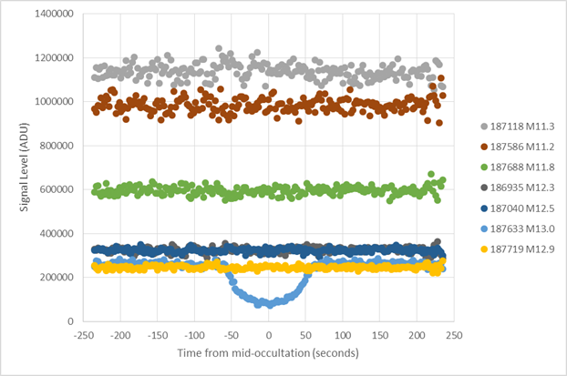
Figure 6. Using the
mean corrections determined from Figure 5, each reference star signal is
plotted over an 8 minute period.
The plots are flat, as expected, and each star has similar noise. The
last six digits of the reference stars from the UCAC4 catalog are used to label
the plots, followed by its magnitude.
The plot of Pluto and the occulted star is also included for reference.
8. Pluto photometric
results
The final, corrected signal level for the target star with Pluto is now calculated and shown in Figure 7. The orange curve is that expected if Pluto had no atmosphere. The occulted value is based on the measured brightness of Pluto and the reference star imaged the previous night, when the star was about 250 pixels from Pluto and at 34.8°altitude (during the occultation, Pluto was at 35.1° altitude, a difference of only 0.3°, or less than 1% of the elevation). That measurement gave the brightness of Pluto as 0.287 that of the occulted star. This corresponds to an occulted magnitude difference of 1.35, ignoring the effect of spectral differences on the sensor, telescope, and differential atmospheric transmission. The nominal visual magnitude difference is 1.4, so this agrees well with the prediction. The ratio of Pluto divided by the sum of Pluto and the occulted star = 0.287/(1+0.287) = 0.223. This is the value plotted in the graph. To reduce noise, the signal was smoothed by using a triangle function (0.25, 0.50, 0.25). This reduces the temporal resolution to 4.48 seconds instead of 2.24 seconds, but this is still small compared to the slow change in the signal. The non-smoothed data is shown in the bottom of Figure 7.
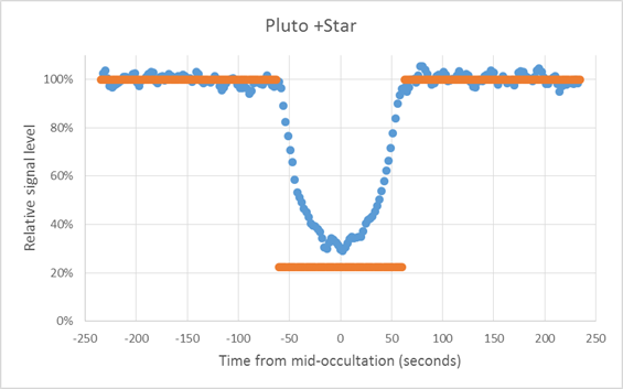
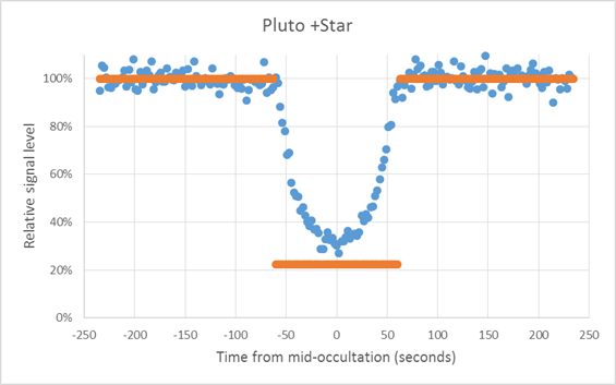
Figure 7. The
normalized intensity of Pluto and the occulted star is plotted over an 8 minute
period. The upper plot is smoothed
to reduce noise, with the raw data plotted in the lower figure. The orange line represents the
transmission predicted if Pluto had no atmosphere.
Note that the curve does not flatten out, indicating a strong atmospheric effect seen even from San Diego, 68% of Pluto’s radius from the center line. The dip is pretty symmetrical; any slight asymmetry may be due to the normalization errors due to the varying transmission (from clouds) during the occultation. The center point in the dimming occurred for image number 358, whose center exposure occurred at 10:32:19.03 pm PDT (UT 05:32:19.03). This is about 4 seconds later than the time predicted by the French Lucky Star project. They also predicted a duration of 93 seconds, where the measured duration was 116 seconds.
This same occulted-brightness ratio calculation was attempted on two sets of measurements made on Aug 14 at 1.47 hours and 1.39 hours before occultation. The atmospheric seeing led to stars about 1.7 arcsec FWHM (after aligning multiple images to reduce noise), or 6 pixels. The separation was 15.5 pixels and 14.2 pixels, respectively, so there was still some overlap between the star and Pluto when using the full Maxim DL apertures. The most careful measurements gave Pluto as 0.33 and 0.31 times as bright as the occulted star, in reasonable agreement with the August 13 measurements. These estimates were not used in the final analysis.
9. Conclusions
The Pluto occultation was successfully imaged from San Diego, about 1200 km north of the center line (830 km projected distance), in spite of some variable clouds over the observation site. The star slowly dimmed for about 60 seconds before reaching a minimum slightly brighter than if Pluto had no atmosphere. No indication of a brightening near the center was observed. The shape of the dimming may give clues to Pluto’s atmosphere, but no further analysis will be presented here.
10. Appendix.
The following figures are from the Lucky Star project, for
reference only. That document was
updated on July 20, 2018 and is found at http://lesia.obspm.fr/lucky-star/predictions/special/pluto20180815.html#sm.
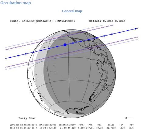
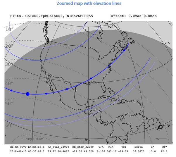
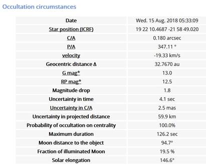
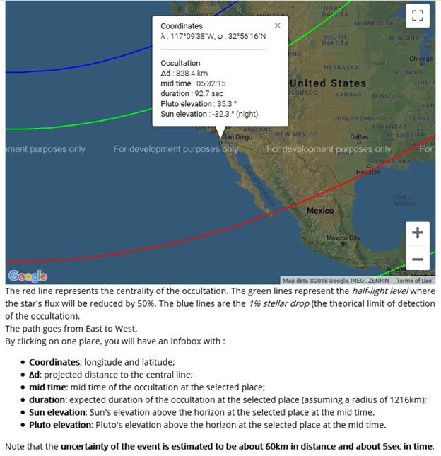
The map includes the
data predictions for the observation site in San Diego.
All text and images are owned by Stellar Products, 1992-2018. Any use by others without permission of Stellar Products is prohibited.
Links to other Stellar Products pages: