Occultations

Occasionally, a planet or asteroid or moon passes in front of a relatively bright star. By measuring the total optical signal using a small telescope, the location of the occulting body can be precisely measured compared to the star. Since the Gaia star catalog is accurate to micro-arcseconds for many stars, the location of the moving body can be measured with similar precision. What is required is a good signal and a good clock. IOTA is the international organization that collects these data from mobile amateur astronomers. Typically, the occultations last a few seconds, so the observer needs to be in the right place at the right time with clear weather. Normally, only a few amateurs have success at each occultation.

Sometimes, however, the path of the occulting shadow happens to fall right over San Diego, so I don’t need to set up at a remote location. Over the past few years, this has happened a few times. The first one I recorded was when Pluto occulted a star in 2018. The second was in 2020, when Jupiter’s largest moon Ganymede occulted a star just at sunset. This was of special interest, since it helped refine Ganymede’s orbit. More recently, I attempted to observe a few other minor asteroid occultations, but I was just outside the shadow. This observing miss does indicate the maximum dimensions of the asteroid.

Click on this link to jump to the Pluto Occultation

Click on this link to jump to the Eurydike Occultation miss

Click on this link to jump to the Hansky Occultation miss

________________________________________________________________________

Ganymede Occultation of Dec 21, 2020 Observed from San Diego

(Written January 5, 2021)

Abstract

The rare occultation of a bright star by Ganymede in December 2020 offered the opportunity to evaluate its current position error as calculated from the JUP357 ephemerides. Since the location of the star (HIP99314) is known to about 50 micro-arcsecond precision from the Gaia DR2 catalog, the timing and path of Ganymede across the star could be determined to a precision only limited by the observation equipment and sky conditions. Based on the 131.3 second +/- 1 second duration of the occultation, the DEC position of Ganymede as determined from the JUP357 ephemerides is in error by about 0.005 arcseconds, with an uncertainty of +/- 0.007 arcseconds. Based on the 0:49:04.5 UT +/- 2 second midpoint time of the occultation, the RA of Ganymede is in error by about 0.0001 arcseconds +/- 0.015 arcseconds. The 2 second uncertainties are estimates based on the noise in the photometric data. These results show that the current ephemerides are adequate to continue the project.

Introduction

An observation project to determine the relativistic deflection of the Galilean moons due to Jupiter’s gravity is aided by knowing the expected location of those moons. There is some controversy over whether these moons will show a relativistic deflection determined by the same equation that applies to stars (0.018 arcsec/J_R, where J_R is the angular distance of the star from Jupiter’s center, measured in units of Jupiter’s radius) or the more complicated equations are necessary, giving deflections about 1000 times smaller and thus not measureable. If the location of one moon within typically 1 J_R is measured with respect to another moon at a further distance from Jupiter, then the relativistic deflection can more easily be determined. This requires the relative locations of the moons to be predicted within 0.002 arcseconds, with a similar accuracy required in the measurements. The question arises if the current JUP357 ephemerides are adequate to predict the location of the moons with this accuracy.

The location of the target moons can be determined by continuously taking images with a telescope and fast CMOS camera, then averaging the locations over a 10-minute series to reduce the measurement noise down to 0.002 arcseconds. This was demonstrated for a series of measurements taken in July 2020 and August 2020 with a stable 200 mm aperture telescope and a cooled CMOS camera. Optical distortion measurements were also recorded using stellar fields, which confirmed the low distortion predicted from optical raytracing. Weather conditions were used to minimize the relative errors, by compensating for atmospheric distortion.

The predicted location of the moons were expected to be on the order of 0.002 arcseconds, based on historical analysis reported in some publications from 1990 to 2010. The JPL/NASA ephemerides for the Galilean moons have recently been updated to JUP357, and the occultation in December 2020 was a good opportunity to verify the current accuracy. For this observation, a larger telescope aperture (280 mm) was used. The occultation occurred in bright twilight, but the data analysis was adequate to complete the experiment.

Method

Table 1 summarizes the equipment and conditions during the transit of Ganymede across HIP99314 seen just after sunset.

Table 1. Parameters for the Ganymede occultation of Dec 20, 2020.

Parameter	Value	Notes
Observing location	San Diego, CA
Observing longitude	W 117 09' 37.0"	Google Earth
Observing latitude	N 32 56' 16.7"	Google Earth
Observing altitude	81 m	Google Earth
Telescope model	Celestron Edge 11	Modified SCT
Telescope aperture	279 mm
Telescope focal length	2800 mm	prime focus
Telescope filter	Atik Red
Telescope filter bandwidth	600 nm to 680 nm
Camera model	ZWO ASI1600MM Pro	CMOS
Camera pixel diameter	3.8 micron square	0.28 arcsecond
Camera gain	5 e-/ADU	12-bit
Image dimension – ROI only	896 (H) x 300 (V)	centered
Camera exposure	0.100 second
Camera software	SharpCap V3.2
Camera frame rate	9.998 fps
Data acquisition start	2020-12-21T00:43:01.054	FITS start time
Data acquisition end	2020-12-21T00:55:01.164	FITS start time
Camera series length	7201 frames
Timing software	Dimension 4 v5.31	Est +/- 0.1 sec
Sun altitude at data recording start	0.217 degree	Guide 9
Sun altitude at mid-occultation	-1.42 degree	Guide 9
Sun altitude at data recording end	-2.53 degree	Guide 9
Ganymede altitude at data recording start	23.78 degree	Guide 9
Ganymede altitude at data recording midpt	22.92 degrees	Guide 9
Ganymede altitude at data recording end	22.06 degrees	Guide 9
Weather temperature at occultation	21.3 C	Wunderground
Weather relative humidity at occultation	35%	Wunderground
Weather barometric pressure at occultation	1025.4 millibar	Wunderground
HIP99314 coordinates (RA, DEC degrees)	302.38957160, -20.59409042	NOVAS J2000

The JPL Horizons web interface was used to predict the location of Ganymede in 1 second intervals, and the separation between Ganymede’s center coordinate and HIP99314 was calculated. The results for the 10 seconds closest to mid-occultation are plotted in Figure 1. At 0:49:04.4 UT the predicted value was 0.3632 arcseconds.

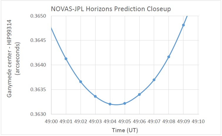
Figure 1. The separation between Ganymede’s center and HIP99314 is plotted as a function of time in 1 second steps. One of the goals of this observation is to confirm this minimum value.

Procedure

The telescope was focused on Ganymede a few minutes before the data acquisition started, with the Sun still above the horizon and the telescope still at the daytime temperature. Because of the low altitude and bright skies, and due to the recent weather pattern, the atmospheric seeing was poor, resulting in a low SNR. This resulted in a relatively poor focus, but since these measurements were photometric instead of astrometric, the performance was deemed acceptable. Over the next 15 minutes, the telescope temperature dropped enough to make the focus slightly worse. Fortunately, the sky also darkened, so the SNR did not deteriorate. A shorter focal length might have produced better data, but a focal reducer was not available.

About an hour before the data acquisition, the laptop computer that controlled the CMOS camera was synchronized use Dimension4 software. The time stamps in the FITS headers that indicate the start of each exposure are estimated to have an uncertainty of 0.1 second. The difference between frame times are accurate to 0.001 seconds. The time between the first frame (G-00001) and the last frame (G-07201) was 720.01 seconds, for a mean of 0.1000014 seconds per frame.

A total of 1000 flat-field frames were saved just before the occultation data started, by pointing the telescope near zenith and slowly moving the pointing angle to prevent stars from appearing. A total of 1000 dark frames were recorded just after the occultation data collection concluded. Both of these sets of data were taken at 0.100 seconds, the same as the occultation series. A master dark and master flat-field were calculated and applied to all of the occultation data. Figure 2 shows the first image frame, stretched to show Callisto (on the far left) and Ganymede surrounded by the measurement annuli.

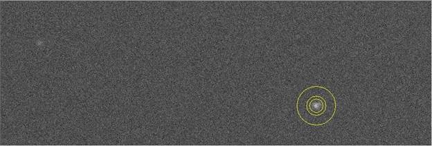
Figure 2. Image G-00001 stretched to show the reference star (Callisto) at the left side and Ganymede + HIP99314 at the right. The signal is measured inside the 14-pixel radius circle after subtracting the mean background measured between the 20-pixel and 40-pixel outer radii. The same measurement radii are used on Callisto. The inner measurement aperture is 8 arcsec in diameter.

Results

A Python program was modified to process the photometric data from each frame. For G-00001, the centroids of Ganymede and Callisto were determined by using MaxIm DL software. The integration radius was set at 14 pixels. Initially, an annulus with inner radius 28 pixels and outer radius 40 pixels was used to determine the background mean, which was subtracted from each pixel used in the central disk. The centroid determined by this set of radii was then used to reposition the measurement annuli (to the nearest pixel) and the final target intensity was measured with a 14-pixel radius and background annuli of 20 and 40 pixels. The location of Callisto was always fixed with respect to Ganymede.

The background level and the RMS background at the frame center was measured over the entire series. Those values are plotted in Figure 3 using a semi-log graph. The sky darkens by a factor of 2.8 over the 12 minutes shown in the graph. The background RMS also falls, but only by a factor of 1.7.

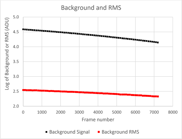
Figure 3. The mean background and background RMS are plotted as a function of time, over a 12 minute period centered on the occultation.

The intensity of Ganymede + HIP99314 is plotted in Figure 4. These points were divided by the Callisto intensity (measured for each frame) to remove sky variations in the signal path, then divided by a factor of 3.5 to normalize the pre-occultation values to 1.00. A black trend line based on a moving average of 30 points is shown to guide the eye. The occultation lasted from about 0:48 to 0:50, in preliminary agreement with the predictions. The mean intensity during the occultation was reduced by about 10%. This value resulted from the red filter wavelength used in the observations.

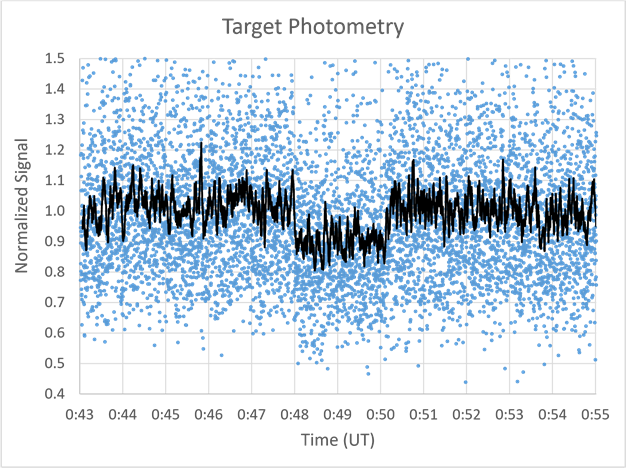
Figure 4. The normalized signal from each frame is plotted as a function of time. The black line is a moving average over 30 points (3 seconds), intended to guide the eye and verify that the occultation was detected near the predicted time.

To mathematically determine the time of disappearance, a least squares calculation was performed, using a single step (1.0 to 0.9) as a function of time. The errors surrounding the disappearance are based on the difference of the intensity and the step-function value from 0:47:31 to 0:48:31. The sums of the squares are plotted in Figure 5, where the disappearance is indicated by the frame number. The best estimate of the disappearance is given by the minimum in the curve at Frame 2978. This corresponds to the time 0:47:58.85. An uncertainty of 0.6 second is used as a reasonable estimate based on a close-up plot of Figure 4.

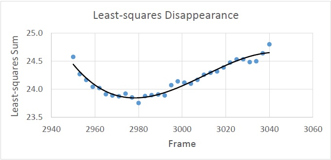
Figure 5. The least-squares calculation of the disappearance is minimized at Frame 2978. Each dot represents a shift in the disappearance by three frames, or 0.3 seconds. A third-order polynomial was fit to the points to determine the minimum sum.

The identical sequence of operations was performed to estimate the reappearance time, shown in Figure 6. Because of a bump in the data just as the signal was increasing, a wider window was used, with a coarser resolution of 1 second. In this case, the best estimate of the reappearance is at Frame 4291, or 0:50:10.2. The uncertainty in this part of the curve is estimated at 2 seconds. The difference between these two times is 131.3 seconds with a center time of 0:49:04.5 and a total uncertainty of 2 seconds. The calculations based on NOVAS on the JUP357 ephemerides was 0:49:04.4, a difference of only 0.1 seconds. This is much smaller than the estimated uncertainty. All of these results are summarized in Table 2.

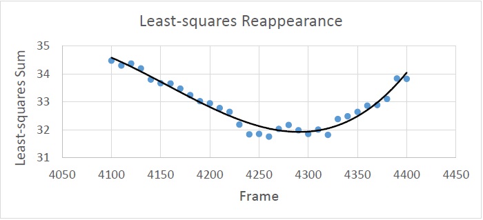
Figure 6. The least-squares calculation of the reappearance is minimized at Frame 4291. Each dot represents a shift in the disappearance by ten frames, or 1.0 seconds. A third-order polynomial was fit to the points to determine the minimum sum.

Table 2. Occultation times, durations, and offsets for predictions and observations.

Parameter	NOVAS/JUP357	Bruns Observation
RA mid-occultation (UT time)	0:49:04.4	0:49:04.5
Occultation duration (seconds)		131.3 +/- 2
DEC closest offset (arcsec)	0.363	0.358 +/- 0.007

The occultation duration measurement can be turned into a DEC offset with a little geometry and assuming the same drift rate. A pass through the center of Ganymede would have taken 161.5 seconds, according to the IOTA chart, so the measured time of 131.3 seconds can be used to calculate the measured offset. The result is 0.358 arcseconds, with a change of 0.007 arcseconds for an uncertainty of 2 second in timing. This DEC difference of 0.005 arcseconds falls well within the uncertainty.

The same close result holds for the timing. The NOVAS/JPL Horizons predicted time for the mid-occultation was 0:49:04.4 and the observed time was 0:49:04.5, a difference of 0.1 seconds in time, much less than the uncertainty. Since the moon moves about 0.0075 arcsec/sec with respect to the stars, a 0.1 second error in time corresponds to an error less than 0.001 arcseconds, and a 2 second uncertainty in time corresponds to a 0.015 arcsecond error in position.

The International Occultation Timing Association (IOTA) made calculations for a nearby location, predicting the center of Ganymede would pass 0.397 arcseconds from the star. Those were based on polynomials used by the French Institute of Celestial Mechanics and Computation of Ephemerides (IMCEE), which have not been updated since 1996. This small difference is not important in setting up the observations around the world, but the September 2020 release of the JPL JUP357 ephemerides seem to be more accurate.

Tony George of Arizona kindly used a Python program called PyOTE, often used in the occultations of asteroids, to re-process this data set. He also adjusted some variables to minimize the uncertainties. His results give an occultation duration of 129.9 seconds +/- 1.9 seconds and a midpoint time of 0:49:03.1. This value leads to a DEC offset of 0.365 arcseconds, which would reduce the measurement error derived from the JUP357 ephemerides to only 0.002 arcseconds. His disappearance time calculation differs by only 0.65 seconds from the time estimated in this paper, and his timing uncertainty also matches the 2 second estimate used earlier. This is considered a good agreement.

Conclusion

The observation here shows that the position of Ganymede, and probably the other Galilean moons, are accurate to within 0.005 arcseconds in DEC, and probably much less than 0.015 arcseconds in RA. The fear was that the ephemerides was not much improved upon earlier versions which had errors on the order of 0.1 arcsecond. Those fears can be ignored, and the JUP357 ephemerides appear to be good enough for the relativistic deflection project to continue.

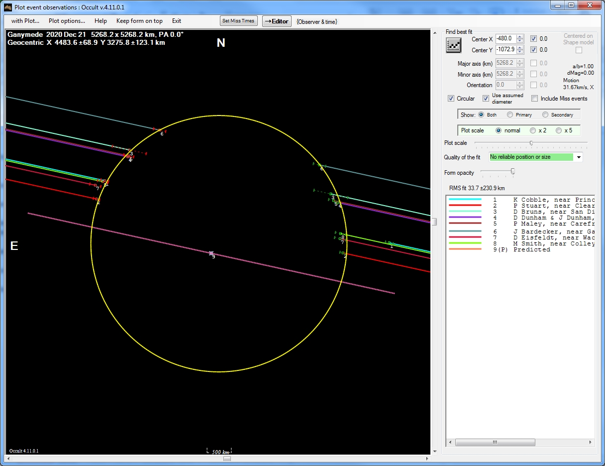
This graph produced by IOTA includes all the observations of this occultation.

___________________________________________________________________________________

Pluto Occultation Observations on 14 August 2018

Abstract

On the evening of August 14, 2018, Pluto slowly occulted a 13^th magnitude star as seen from San Diego. Using a 28 cm aperture telescope with a CMOS camera, the photometric brightness of the combined star and Pluto was recorded over 27 minutes using 2 second exposures separated by 0.24 seconds. The brightness was calibrated by using six nearby reference stars in the same images, which compensated for some variable clouds that affected the raw measurements. The greatest dimming occurred at 10:32:19 pm PDT and the dimming lasted 116 seconds. This is 4 seconds later and 23 seconds longer than predicted.

1. Introduction

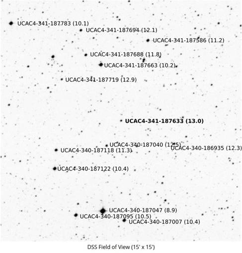
On August 14, 2018, a few hours after sunset in San Diego, Pluto crossed in front of UCAC4-341-17633, a 13^th magnitude star. Since Pluto was about magnitude 14.4, the total light from both targets dropped to about 20% of the light before and after the occultation. A telescope was used to collect enough light to record a time series of images. Pluto’s atmosphere scattered some light as the star passed behind Pluto, so the dimming was not instantaneous.

This photometric data was desired by the Lucky Star astronomical group headquartered in France, who coordinated the effort to get observers all across the shadow of Pluto as it crossed across North America (see figures in the Appendix). San Diego was about midway from the centerline to the edge, but Pluto was on the meridian at 35° altitude.

The equipment used for data acquisition is shown in Table 1. No color filters were included. The 1.7 arcsec seeing produced stellar images about 6 pixels FWHM. The sensor rows were oriented parallel to celestial Right Ascension. SharpCap was used to run the camera and MaxIm DL was used to process the images. Each image is time-stamped in the software at the time the exposure ended, so one second was subtracted to get the center time. There is an uncertainty of about 0.2 seconds because of the time stamping process, but this is negligible compared to the time seen in the occultation dip.

Table 1. Equipment parameters

Parameter	Value	Comment
Telescope	28 cm aperture	Celestron Edge C11 at F/9.7
Mount	German equatorial	Software Bisque MyT Paramount
Camera	CMOS monochrome, cooled	ZWO ASI1600MM PRO
Plate scale	0.288 arcsec/pixel	3.8 μm pixel, 2722 mm focal length
FOV	23 x 17 arcmin	4656 x 3520 pixels
Image dead time	0.236 seconds	Download and save

The night before the occultation, at about the same time, calibration images were recorded. Pluto was far enough from the target star that good relative brightness measurements could be calculated. This brightness ratio was used in the final data analysis.

To calibrate the camera and optical system, twilight flat field images were recorded on Aug 14. Since the camera was temperature controlled at - 10 C, dark frames from August 13 were used. During the occultation, some low clouds started to appear which reduced the sky transparency. Fortunately, the sky was clear enough during the event to complete the data acquisition, and six reference stars surrounding Pluto were averaged to calibrate the data.

2. Dark field images

On August 13, 2018, 200 dark images were recorded by covering the telescope aperture during twilight (starting at 7:45 pm PDT, when the Sun was 3° below the horizon). Series were taken with the gain set to 200, 220, and 250, since the gain during the occultation was not yet determined. The exposure times were 0.012 sec (as used in the twilight flat frames) and 2 seconds (as used for the Pluto images). The 2 sec darks were taken starting at about 8 pm (Sun at -6°). The CMOS camera cooler was set at -10 C, using typically 25% power, so the temperature was stable. The actual temperature readout was noted as varying from -10 C to -10.5 C, an insignificant effect on the dark noise. The ZWO camera digitizes using 12-bits, and are automatically shifted two bits to get a range from 0 to 64k in 16 ADU steps. Each image file is 32MB.

All images were stacked using MaxIm DL software, with no alignment shift, using simple averaging. The saved files are considered master images, and were labelled DARK12msG200mean200, DARK12msG220mean200, DARK12msG250mean200, DARK2sG200mean200, DARK2sG220mean200, and DARK2sG250mean200. All master files are saved in FITS format, using IEEE Floating numbers, resulting in 64MB files. These are used to correct the image files taken on August 14, since the electronics are temperature controlled. Similar dark frames from August 12 had the same RMS noise.

Single image noises for the combinations are in Table 2. The noise does not diminish as the square root of the number of frames, so some fixed-pattern noise is present.

Table 2. Image noise for various exposure and camera gain combinations.

Configuration exposure (msec)	Configuration gain	RMS noise (ADU) in single image	RMS noise (ADU) in average of 200 images
12	200	47	9.7
12	220	55	11.8
12	250	75	16.6
2000	200	55	20
2000	220	65	25
2000	250	89	35

3. Flat-field images

On August 14, 2018, flat-field images were recorded by pointing the telescope near the meridian at about 40° elevation just at sunset (first ones starting at 7:33 pm PDT). Starting with the 200 gain setting, a total of 200 images were taken. The gain was increased to 250 as the sky darkened. During the exposures, the telescope was moving at about 45 arcsec/sec in Declination (using the manual joystick). By the time each sequence was completed, the pointing was direction was shifted by more than a field of view, preventing any possible star buildup. The camera cooler was set at -10 C, typically using 25% power, assuring a stable temperature.

All images were stacked in MaxIm DL with no alignment shift, using simple averaging. A master dark frame was subtracted to complete the calibration. The files were saved as FLATG200E12ms_mean200, FLATG220E12ms_mean200, and FLATG250E12ms_mean200. Figure 1 shows the resulting flat field image (stretched for more contrast) and a horizontal profile through the center. There is one dust donut slightly left of center and a few smaller ones on the right side, but all are far from any reference stars.

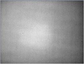
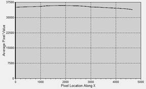
Figure 1. (Left) Flat field image, stretched to show the uniformity across the field. No dust shadows fell near the reference stars. (Right) A horizontal profile plot near the center shows the signal at the edges falls only a few percent compared to the center.

4. Pluto image collection

After the flat field images were completed at 7:40 pm, the telescope was idle until 8:45 pm. The telescope was centered on Pluto and the pointing was not changed over the evening. The telescope was carefully focused using magnitude 8.9 star UCAC4-340-187047 using exposures about 0.2 seconds. This allowed a real-time display to ease focusing through the turbulence. The air temperature was 69° F and stayed at this number all during this first series. The reference star UCAC4-341-187663 at magnitude 10.2 was then monitored for saturation, after setting the exposure time to 2 seconds. The gain was set so that this star was just under saturation, by watching the display for about 100 frames. It turns out that since the seeing was variable, some of the frames did end up close enough to saturation that some non-linearity showed up, so this star was not used in the final analysis. The brightest reference star used in the final analysis was UCAC4-340-187118 at magnitude 11.3.

The first Pluto image series was started at 9:01 pm, when Pluto was about 15.5 pixels from UCAC4-341-187633, the occulted star. The intent was to use this series to measure the relative signals of the two objects to high precision, but as explained later, this series was only good enough to estimate the ratio. The seeing blurred the star and Pluto too broadly to allow better results. Nevertheless, 155 images (with 2 second exposures) were recorded using a gain of 200 and another series of 100 at a gain of 220. This imaging series ended at 9:10 pm. Starting at 9:22, the same focus and gain tests were repeated, with the image series starting at 9:31 pm and ending at 9:33 pm. The gain was set at 220, and the temperature was stable at 69° F.

At 10:08 pm, the laptop was time-synchronized using Dimension 4 software that connects with an accurate internet time server. Some low clouds were approaching Pluto, so the camera gain was increased to 250. During focus and gain testing, the temperature was 68° F, and stayed at this value until the data collection ended. The image series started at 10:19 pm and ended at 10:46 pm. The occultation occurred at 10:32 pm, but the 27 minute long series allowed a better monitor of the cloud cover. It was too cloudy to take a planned series of images with Pluto on the opposite side of the target star one hour later.

5. Image corrections

The following steps were performed on every final Pluto sky image. The appropriate master dark image was subtracted while adding 1000 ADU to prevent negative values. The files were renamed by appending –dark. (For the flat fields, the additional 1000 ADU offset was not used.)

The flat fields were renormalized by dividing by the mean (which was calculated over the entire image), resulting in nearly every pixel varying between typically 1.04 in the center to 0.94 in the corners. In the central region, near Pluto and the reference stars, the mean values vary between 1.00 and 1.02. These files were renamed to FLATG200E12ms_mean200-meandark-normto1, FLATG220E12ms_mean200-meandark-normto1, and FLATG250E12ms_mean200-meandark-normto1.

Every Pluto image was then divided by the appropriate normalized file. Because those dark-subtracted files had an additional 1000 ADU added, one more step was required. A constant image, where every pixel was set to 1000 ADU, was created and divided by the normalized flat field image. At the same time, an additional 1000 ADU was added to prevent negative values. Mathematically, this is explained by:

(RAW-DARK-1000) - 1000 ₌ (RAW-DARK)

NORM(FLAT) NORM(FLAT) NORM(FLAT).

Since the intensity of the target and reference stars are determined in MaxIm DL by the sum of the pixel values inside a circular area minus the mean value of the pixels in a surrounding annulus, the absolute level is not important.

The flatness across a typical image is shown in Figure 2. The upper trace labelled “Raw” is a horizontal profile across the image, averaged over 20 pixels to reduce noise. One star shows up in the data. The curve is normalized to 1 and shifted up by 0.05 to show the general slope. The lower trace labelled “Raw/FF” is the same data with each pixel divided by the flat field curve, offset by -0.05. The shape is over-corrected because of the additional 1000 ADU offset meant to eliminate negative values. The middle trace labelled “Raw/FF-1000/FF” is the final result to which the photometry will be applied. This curve is very flat, as expected.

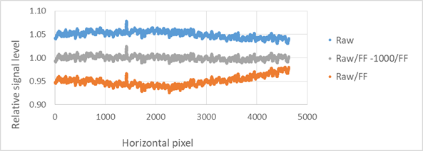
Figure 2. The flat field correction is shown by horizontal plots of the normalized intensity for the raw image, an intermediate image, and the final corrected image. The final image is flat to better than 1%.

6. Integrated Signal Measurements

MaxIm DL integrates the ADU signal inside a circle of radius R1, then subtracts the mean signal background determined from an annulus with outer radius radii R2. If the radii are too large, excess noise is added, so the optimum diameter was determined using several images with FWHM varying from 4.9 to 6.3 pixels. Tests were done on the target star (with Pluto just a few minutes before occultation) and a bright reference star. Varying the inner radius R1 while keeping the outer radius R2 fixed at 19 pixels resulted in the plot in Figure 3. With an R1 of 9 pixels, 95% of the integrated signal is captured, and that fraction varies only by about 1% over the different test stars. This is the radius used for all intensity analysis.

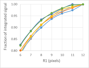
Figure 3. Increasing the aperture around a star collects more light with the penalty of increasing noise. Using an aperture of 9 pixels collects 95% +/- 1% of the total light, and is the radius used in all of the processing.

The process to easily copy the integrated intensities for hundreds of images in a series was the following. Every full image was opened and cropped and saved to a smaller image with 250x150 pixels dimensions, with the image center around one of six reference stars or Pluto. In this way, all 722 images in the time series could be opened at once, without computer memory problems. The MaxIm DL ALIGNMENT process was started, choosing “Auto one star”. The program took just a few seconds to align all of the images with respect to the first chosen reference image, using the bicubic interpolation option to estimate the new shifted pixel values. The process was closed, then re-opened, choosing “NONE” for alignment. The cursor was set at R1=9 and R2=19, simply advancing to the next image after manually copying the intensity value into an Excel spreadsheet. No realignment between images was needed, and the values are within 0.1% when compared to the original images.

7. Sky transmission results

The relative sky transmission over the entire 27 minute occultation observation series was estimated by measuring the signal intensity of one nearby star (UCAC4-340-187118) in each of 722 images. At magnitude 11.3, its peak pixel was typically between 20,000 and 30,000 ADU, well within the linear range. The signal from the unresolved target star UCAC4-341-187633 and Pluto was also measured for each image. Both signals were normalized to 100% for the images taken about 700 seconds after the occultation, where the maximum transparency was seen. The results are plotted in Figure 4. The relative transparency dropped to about 40% at the beginning of the occultation, and rapidly increased to 75% during the occultation. Because several reference stars on both sides of the target star were measured, this drop should not affect the final results. The transmission was compared to images taken on the previous day, when no clouds were noted; the transmission was essentially identical. This means that the 100% level indicated in the figure represents a clear sky with some low-level haze.

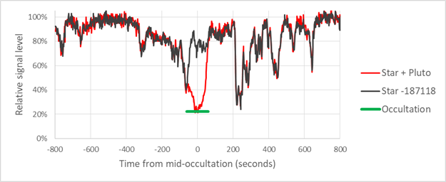
Figure 4. The change in the sky transparency is plotted over a 1600 second period centered on the occultation. The black curve is the signal from a nearby reference star and the red line is the signal from Pluto and the star it occulted. The time of the occultation is indicated by the green bar. The signals are normalized to 100% at 700 seconds, where the transmission was greatest.

Images taken just before and after the occultation were analyzed to give a better mean value for the relative atmospheric transmission across the image during this critical time period. Since the clouds were moving, it was assumed that averaging the transmissions over several reference stars surrounding Pluto would reduce the noise and give a smoother result. These results are plotted in Figure 5, showing the relative transmissions for the six stars used in the analysis. The simple mean was used in the final analysis with no weighting by SNR, since the SNRs for each star were always much greater than 50.

Figure 5. The relative signal strength of six stars near Pluto was measured over an 8 minute period centered on the occultation. Averaging these measurements gives a better mean transmission factor.

With this mean transmission function, the signal levels for the six reference stars and the target star could be calculated. The results are shown in Figure 6. The intensity as a function of time is flat for all reference stars, as expected. The RMS of each star divided by the mean level ranges between 0.023 and 0.030, with an average RMS/mean of 0.026. This is for data at the 2.24 second recording rate, not smoothed over time.

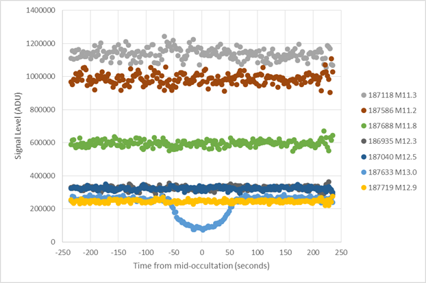
Figure 6. Using the mean corrections determined from Figure 5, each reference star signal is plotted over an 8 minute period. The plots are flat, as expected, and each star has similar noise. The last six digits of the reference stars from the UCAC4 catalog are used to label the plots, followed by its magnitude. The plot of Pluto and the occulted star is also included for reference.

8. Pluto photometric results

The final, corrected signal level for the target star with Pluto is now calculated and shown in Figure 7. The orange curve is that expected if Pluto had no atmosphere. The occulted value is based on the measured brightness of Pluto and the reference star imaged the previous night, when the star was about 250 pixels from Pluto and at 34.8°altitude (during the occultation, Pluto was at 35.1° altitude, a difference of only 0.3°, or less than 1% of the elevation). That measurement gave the brightness of Pluto as 0.287 that of the occulted star. This corresponds to an occulted magnitude difference of 1.35, ignoring the effect of spectral differences on the sensor, telescope, and differential atmospheric transmission. The nominal visual magnitude difference is 1.4, so this agrees well with the prediction. The ratio of Pluto divided by the sum of Pluto and the occulted star = 0.287/(1+0.287) = 0.223. This is the value plotted in the graph. To reduce noise, the signal was smoothed by using a triangle function (0.25, 0.50, 0.25). This reduces the temporal resolution to 4.48 seconds instead of 2.24 seconds, but this is still small compared to the slow change in the signal. The non-smoothed data is shown in the bottom of Figure 7.

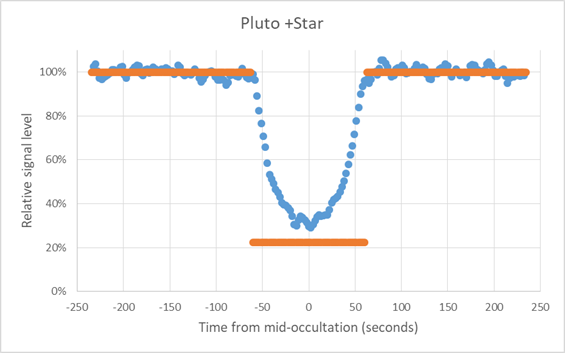
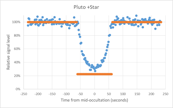
Figure 7. The normalized intensity of Pluto and the occulted star is plotted over an 8 minute period. The first plot is smoothed to reduce noise, with the raw data plotted in the second figure. The orange line represents the transmission predicted if Pluto had no atmosphere.

Note that the curve does not flatten out, indicating a strong atmospheric effect seen even from San Diego, 68% of Pluto’s radius from the center line. The dip is pretty symmetrical; any slight asymmetry may be due to the normalization errors due to the varying transmission (from clouds) during the occultation. The center point in the dimming occurred for image number 358, whose center exposure occurred at 10:32:19.03 pm PDT (UT 05:32:19.03). This is about 4 seconds later than the time predicted by the French Lucky Star project. They also predicted a duration of 93 seconds, where the measured duration was 116 seconds.

This same occulted-brightness ratio calculation was attempted on two sets of measurements made on Aug 14 at 1.47 hours and 1.39 hours before occultation. The atmospheric seeing led to stars about 1.7 arcsec FWHM (after aligning multiple images to reduce noise), or 6 pixels. The separation was 15.5 pixels and 14.2 pixels, respectively, so there was still some overlap between the star and Pluto when using the full Maxim DL apertures. The most careful measurements gave Pluto as 0.33 and 0.31 times as bright as the occulted star, in reasonable agreement with the August 13 measurements. These estimates were not used in the final analysis.

9. Conclusions

The Pluto occultation was successfully imaged from San Diego, about 1200 km north of the center line (830 km projected distance), in spite of some variable clouds over the observation site. The star slowly dimmed for about 60 seconds before reaching a minimum slightly brighter than if Pluto had no atmosphere. No indication of a brightening near the center was observed. The shape of the dimming may give clues to Pluto’s atmosphere, but no further analysis will be presented here.

10. Appendix.

The following figures are from the Lucky Star project, for reference only. That document was updated on July 20, 2018 and is found at http://lesia.obspm.fr/lucky-star

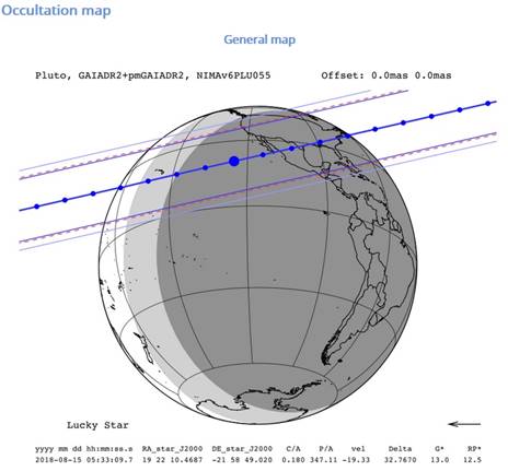
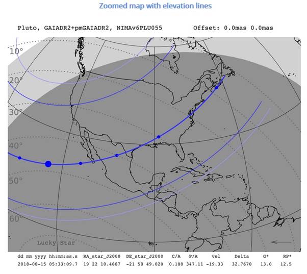
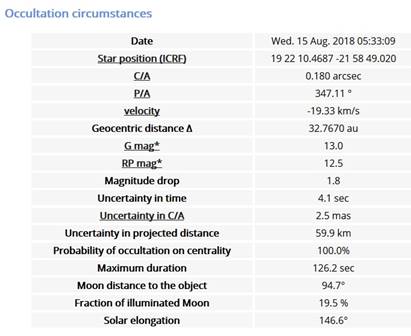
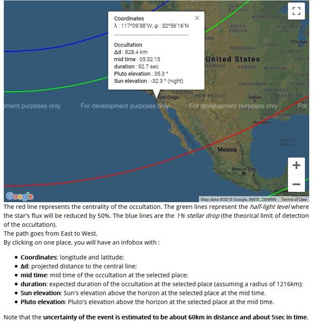
The map includes the data predictions for the observation site in San Diego.

Observations of Asteroid Occultation on March 31, 2021

(written March 31, 2021)

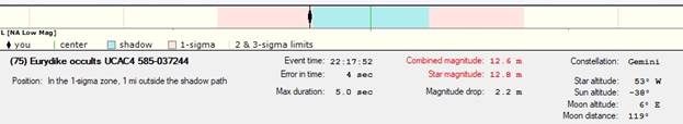
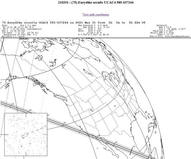
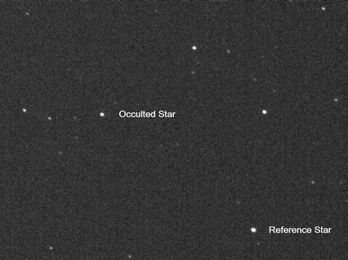
Asteroid 75 Eurydike occulted a mag 12.8 star just after 10 pm (PDT) March 30, 2021 (March 31 UT). I used a 200mm Ritchey-Chretien telescope at F/8 with a ZWO1600 CMOS camera to capture the asteroid, target star, and possible occultation. From the OccultWatcher program, my location was only about 1 mile from the predicted shadow edge, with an uncertainty of 5 miles. The target star, combined with the asteroid, should show a brightness drop to about 20% of the star’s normal amplitude. The star is dim, but was successfully imaged using 333 msec exposures, with an SNR close to 15, when the camera gain was set to 300 (0.16 electrons/ADU). No filter was used in front of the camera. Using 5 second exposures and combining 30 images, stars down to magnitude 17 were visible. The star field was imaged this way at 8pm, 9pm, 10pm, and 10:40pm (PDT) and the combined series were annotated here. The 14.8 magnitude asteroid is easily seen. The Reference star (TYC 1904 217) at mag 10.2 was used to normalize the signal from the target star. At this exposure, its signal was about one-half of the full well. The seeing produced images about 2 arcsec FWHM, and the local humidity was 97% during the event. Between the short test series, the telescope was covered with a white towel and a heater with a fan behind the primary was turned on. The image quality recovered about 10 minutes after the fan and heater were turned off. During the event, the telescope was pointed over the nearby neighbor’s home, which slight affected the seeing.

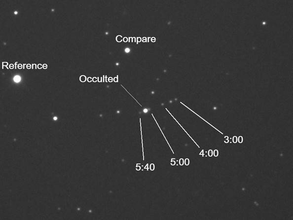
The target was imaged using SharpCap with a 333msec exposure, with essentially no overhead time. The laptop was synchronized using Dimension4 software, to about 0.1 seconds, at 10pm. This fast series started at 10:16pm and lasted 4 minutes. The expected occultation should have occurred at 10:17:52 pm, but nothing was seen. The graph shows the target star in blue, with horizontal lines at the +/- 3 sigma level. For comparison, a nearby comparison star that was 1.5 times brighter, was also processed, shown with its +/- 3 sigma levels. This data was measured frame-by frame using MaxIm DL with aperture radius 10 pixels (4.8 arcseconds radius) and a background annulus with inner radius 17 pixels and outer radius 29 pixels. The bright star shown at the left in the figure was used to normalize the signal intensities, although no clouds were present. That star had a signal variation of about 4%, while the target star varied by about 9%. The comparison star has an RMS of about 7%.

The occultation occurred at 5:17:52 in San Diego, with an uncertainty of 4 seconds.

If the asteroid occulted the star for longer than 0.333 seconds, then the signal would have dropped to about 0.15. Since this was not seen, any occultation would have had to last less than about 0.1 second. Based on the asteroid speed of about 12 km/sec, any moon or asteroid edge would have to be less than about 1 km diameter to be detected. The dip at 5:17:57 is probably just a statistical artifact.

The following charts are from the OccultWatcher program.

A75 map2

A75 map

__________________________________________________________________________________________________

Observations of Asteroid Occultation on April 30, 2021

(written April 30, 2021)

Asteroid 1118 Hanskya was predicted to occult a mag 11.9 star at 21:40:31 (PDT) April 29, 2021 (April 30 UT). I used a 200mm Ritchey-Chretien telescope at F/8 with a ZWO1600 CMOS camera to capture the target and reference stars. From the OccultWatcher program, my location was 1.2 km inside the predicted shadow edge, with an uncertainty of about 1.5 km. The target star, combined with the asteroid, should show a brightness drop to about 2% of the star’s normal amplitude. The star is dim, but was successfully imaged using 200 msec exposures, with an SNR close to 15, when the camera gain was set to 250 (~0.2 electrons/ADU). No filter was used in front of the camera. A combined series of 10 images is annotated here. The Reference star (TYC 1891 901) at mag 11.2 was used to monitor the signal from the target star. At this exposure, its peak pixel value was about 4% of the 16-bit limit, well below saturation. The seeing produced images about 2.5 arcsec FWHM, and the local humidity was 40% during the event. During the event, the telescope was pointed over the nearby neighbor’s home, which slightly affected the seeing. The other two bright stars were also analyzed, and they also remained constant.

The target was imaged using SharpCap with a 200 msec exposure, with essentially no overhead time. The laptop was synchronized using Dimension4 software, to about 0.1 seconds, at 21:30. This fast series started at 21:38 and lasted 4 minutes. The expected occultation should have occurred at 21:40:31 pm, at +31 seconds in the graph, but no drop was seen. The graph shows the integrated signal for the target star in orange. For comparison, the graph also plots the signal from the Reference star, which was twice as bright. This data was measured frame-by frame using a Python program with aperture radius of 10 pixels (4.8 arcseconds radius). The Reference star dip at 4:39:10 UT did not occur in the other, slightly dimmer reference stars.

The occultation occurred at 4:40:31 UT near San Diego, with an uncertainty of 1 second.

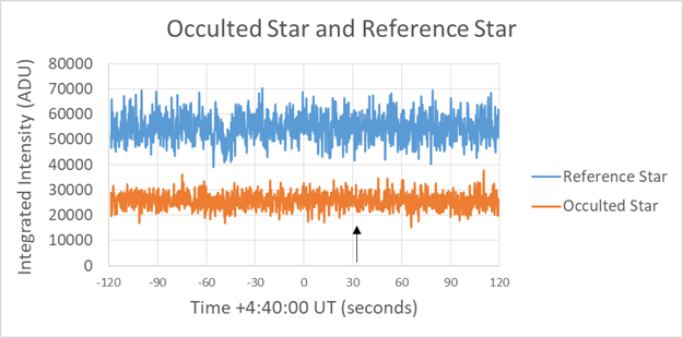
The time sequence near the predicted occultation is shown in the next graph, with horizontal lines at the +/- 3 sigma level (determined over the entire 4 minute interval). Based on the predicted shadow edge at 1.2 km from my site, the expected dip for a spherical asteroid would have lasted 0.60 seconds, or 3 points. Based on the noise level, any occultation was less than about 0.05 seconds. This measurement indicates the asteroid is either not spherical, or the uncertainty in the prediction was realized.

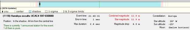
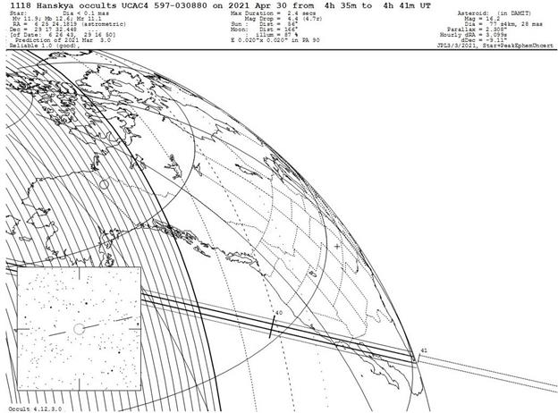
The following charts are from the OccultWatcher program.

prediction map

Thank you for your interest in Stellar Products!

All text and images are owned by Stellar Products, 1992-2021. Any use by others without permission of Stellar Products is prohibited. For information on commercial use of any of these images, click here.

Web page last updated May 4, 2021.